Difference between revisions of "Format notes"
(→Images) |
(→Categories) |
||
| (28 intermediate revisions by the same user not shown) | |||
| Line 1: | Line 1: | ||
This is a list of common code templates and styles we use at specialfunctionswiki. | This is a list of common code templates and styles we use at specialfunctionswiki. | ||
| + | |||
| + | =Defining a new function= | ||
| + | Try to follow roughly the following as much as possible: | ||
| + | <pre> | ||
| + | The such-and-such function $\mathrm{mathname} \colon domain \rightarrow codomain$ is defined by | ||
| + | $$\mathrm{mathname}(x) = 2 \displaystyle\int_a^x t\mathrm{blabla}(t) \mathrm{d}t,$$ | ||
| + | where $\mathrm{blabla}$ is the [[blabla]] function. | ||
| + | </pre> | ||
| + | which generates: <br /> | ||
| + | The such-and-such function $\mathrm{mathname} \colon domain \rightarrow codomain$ is defined by | ||
| + | $$\mathrm{mathname}(x) = 2 \displaystyle\int_a^x t\mathrm{blabla}(t) \mathrm{d}t,$$ | ||
| + | where $\mathrm{blabla}$ is the [[blabla]] function. | ||
=Theorem/proof box template= | =Theorem/proof box template= | ||
| + | ==New way== | ||
| + | Each theorem should have its own page. Each theorem page should be formatted in the following way: | ||
| + | <pre> | ||
| + | __NOTOC__ | ||
| + | |||
| + | ==Theorem== | ||
| + | statement of theorem | ||
| + | |||
| + | ==Proof== | ||
| + | proof of theorem █ | ||
| + | |||
| + | ==References== | ||
| + | references to this fact in the literature | ||
| + | |||
| + | [[Category:Theorem]] | ||
| + | </pre> | ||
| + | |||
| + | ==Old way== | ||
| + | The following code that appears in many places should be phased out in favor of the above. | ||
| + | |||
The code | The code | ||
<pre><div class="toccolours mw-collapsible mw-collapsed"> | <pre><div class="toccolours mw-collapsible mw-collapsed"> | ||
| − | <strong> | + | <strong>Theorem:</strong> STATEMENT OF THEOREM |
<div class="mw-collapsible-content"> | <div class="mw-collapsible-content"> | ||
<strong>Proof:</strong> proof goes here █ | <strong>Proof:</strong> proof goes here █ | ||
| Line 11: | Line 43: | ||
creates | creates | ||
<div class="toccolours mw-collapsible mw-collapsed"> | <div class="toccolours mw-collapsible mw-collapsed"> | ||
| − | <strong> | + | <strong>Theorem:</strong> STATEMENT OF THEOREM |
<div class="mw-collapsible-content"> | <div class="mw-collapsible-content"> | ||
<strong>Proof:</strong> proof goes here █ | <strong>Proof:</strong> proof goes here █ | ||
| Line 35: | Line 67: | ||
</div> | </div> | ||
| − | |||
==Domain colorings== | ==Domain colorings== | ||
| + | In Ubuntu... modify the cplot function in | ||
| + | <pre>/usr/lib/python2.7/dist-packages/mpmath/visualization.py</pre> | ||
| + | by commenting out the if statement at the end as follows: | ||
| + | <pre> | ||
| + | #if fig: | ||
| + | # if file: | ||
| + | # pylab.savefig(file, dpi=dpi) | ||
| + | # else: | ||
| + | # pylab.show() | ||
| + | </pre> | ||
| + | |||
| + | This will allow us to call the savefig function ourselves as we do below. You may also alter the savefig command in visualization.py to have the correct parameters, but in most domain colorings we won't assume this. | ||
| + | |||
| + | ===With Python (best way)=== | ||
| + | We modify the code | ||
| + | <pre>#!/usr/bin/python | ||
| + | import numpy as np | ||
| + | import matplotlib.pyplot as plt | ||
| + | from mpmath import * | ||
| + | |||
| + | cplot(lambda sin(x): f(x),[-10,10],[-10,10],points=50000,verbose=True) | ||
| + | plt.savefig('complexsinedomaincoloring.png',bbox_inches='tight',pad_inches=0.0)</pre> | ||
| + | |||
| + | to generate domain colorings. | ||
| + | |||
| + | ===With Mathematica (old way)=== | ||
We use the code | We use the code | ||
<pre>ComplexGraph[f_, {xmin_, xmax_}, {ymin_, ymax_}, | <pre>ComplexGraph[f_, {xmin_, xmax_}, {ymin_, ymax_}, | ||
| Line 52: | Line 109: | ||
<pre> f[z_]:=z | <pre> f[z_]:=z | ||
ComplexGraph[f,{-10,10},{-10,10}]</pre> | ComplexGraph[f,{-10,10},{-10,10}]</pre> | ||
| − | |||
| − | |||
| − | == | + | ==Glyphs== |
| + | When uploading a glyph (whether a plot in the plane or a domain coloring or a 3d graph), put <pre>[[Category:functionnameglyph]]</pre> in the description. | ||
| + | |||
| + | ===With Python (best way)=== | ||
| + | We use [http://mpmath.org/ mpmath] with the file visualization.py (in Debian, it is located at /usr/lib/python2.7/dist-packages/mpmath/visualization.py) altered in the following way: comment the two following lines | ||
| + | <pre>axes.set_xlabel('Re(z)') | ||
| + | axes.set_ylabel('Im(z)')</pre> | ||
| + | and add the following line | ||
| + | <pre>axes.set_axis_off()</pre> | ||
| + | Doing this will get rid of the left and right matter when using cplot. After this, use an image editing program (such as [https://www.gimp.org gimp]) to cut out a square in the colored region. Upload this raw square with a filename like "complexsineglyph.png" (use prefix complex for domain colorings, without that prefix it should refer to a normal plot-type glyph) and upload that file. | ||
| + | |||
| + | ====$y=f(x)$-type graphs==== | ||
| + | <pre>#!/usr/bin/python | ||
| + | import numpy as np | ||
| + | import matplotlib.pyplot as plt | ||
| + | from mpmath import * | ||
| + | from pylab import rcParams | ||
| + | rcParams['figure.figsize'] = 2.4,2.4 | ||
| + | |||
| + | x=np.arange(0,2*pi,0.00001) | ||
| + | f=np.vectorize(sin) | ||
| + | y=f(x) | ||
| + | |||
| + | fig, ax = plt.subplots() | ||
| + | plt.ylim([-1.1,1.1]) | ||
| + | #ax.spines['left'].set_position('center') | ||
| + | ax.spines['right'].set_color('none') | ||
| + | ax.spines['bottom'].set_position('center') | ||
| + | ax.spines['top'].set_color('none') | ||
| + | ax.spines['left'].set_smart_bounds(True) | ||
| + | ax.spines['bottom'].set_smart_bounds(True) | ||
| + | ax.xaxis.set_ticks_position('none') | ||
| + | plt.tick_params(axis='x', which='both', bottom='off', top='off', labelbottom='off') | ||
| + | plt.tick_params(axis='y', which='both', left='off', right='off', labelleft='off') | ||
| + | |||
| + | plt.plot(x,y,linewidth=5,color='Black') | ||
| + | |||
| + | plt.savefig('sineglyph.png',bbox_inches='tight',pad_inches=0.0) | ||
| + | </pre> | ||
| + | generates | ||
| + | [[File:Sineglyph.png]]<br /> | ||
| + | which we upload to the Wiki with name sineglyph.png. The file we get is [[File:Sineglyph.png]] -- notice we have added the category | ||
| + | <pre>[[Category:sineglyph]]</pre> | ||
| + | This is so that we can use the randomimagebycategory extension. | ||
| + | |||
| + | ====Domain colorings==== | ||
| + | We use [http://mpmath.org/ mpmath] with the file visualization.py altered in the following way: comment the two following lines | ||
| + | <pre>axes.set_xlabel('Re(z)') | ||
| + | axes.set_ylabel('Im(z)')</pre> | ||
| + | and add the following line | ||
| + | <pre>axes.set_axis_off()</pre> | ||
| + | Doing this will get rid of the left and right matter when using cplot. After this, use an image editing program (such as [https://www.gimp.org gimp]) to cut out a square in the colored region. Upload this raw square with a filename like "complexsineglyph.png" (use prefix complex for domain colorings, without that prefix it should refer to a normal plot-type glyph) and upload that file. | ||
| + | |||
| + | ===With Mathematica (old way)=== | ||
We use the Mathematica code | We use the Mathematica code | ||
<pre>Plot[AiryAi[x], {x, -12, 3}, PlotStyle -> {Thickness[0.04], Black}, AxesStyle -> Thickness[0.01], Ticks -> None]</pre> | <pre>Plot[AiryAi[x], {x, -12, 3}, PlotStyle -> {Thickness[0.04], Black}, AxesStyle -> Thickness[0.01], Ticks -> None]</pre> | ||
| Line 66: | Line 174: | ||
=Extensions= | =Extensions= | ||
| + | ==RandomImageByCategory== | ||
We use a modified version of [https://www.mediawiki.org/wiki/Extension:RandomImageByCategory RandomImageByCategory]: inside RandomImageByCategory.php, replace the line | We use a modified version of [https://www.mediawiki.org/wiki/Extension:RandomImageByCategory RandomImageByCategory]: inside RandomImageByCategory.php, replace the line | ||
<pre>$thumbnail = "<a href=\"" . htmlspecialchars( $image_title->getFullURL() ) . "\">{$thumb_image->toHtml()}</a>";</pre> | <pre>$thumbnail = "<a href=\"" . htmlspecialchars( $image_title->getFullURL() ) . "\">{$thumb_image->toHtml()}</a>";</pre> | ||
| Line 74: | Line 183: | ||
This prevents RandomImageByCategory from forcing the generated image to link to the image itself and allows you make a randomly generated image link to another page using the following code: | This prevents RandomImageByCategory from forcing the generated image to link to the image itself and allows you make a randomly generated image link to another page using the following code: | ||
<pre>[[Sine|<randomimagebycategory categories="Sineglyph" width="45" />]]</pre> | <pre>[[Sine|<randomimagebycategory categories="Sineglyph" width="45" />]]</pre> | ||
| − | generates the randomly chosen image from the category Sineglyph | + | generates the randomly chosen image from the category [[:Category:Sineglyph]]: |
[[Sine|<randomimagebycategory categories="Sineglyph" width="45" />]] | [[Sine|<randomimagebycategory categories="Sineglyph" width="45" />]] | ||
| + | |||
| + | =Categories= | ||
| + | When uploading a traditional $x$-axis $y$-axis plot, use <pre>[[Category:Plot]]</pre> | ||
| + | When uploading a domain coloring, use | ||
| + | <pre>[[Category:DomainColoring]]</pre> | ||
| + | For any page for a specific special function, use | ||
| + | <pre>[[Category:SpecialFunction]]</pre> | ||
| + | When making a new theorem, use | ||
| + | <pre>[[Category:Theorem]]</pre> | ||
| + | If a theorem is proven, use | ||
| + | <pre>[[Category:Proven]]</pre> | ||
| + | If a theorem is not proven, use | ||
| + | <pre>[[Category:Unproven]]</pre> | ||
| + | If a theorem's proof requires more justification to be technically rigorous, then add the following category in addition to "Category:Theorem": | ||
| + | <pre>[[Category:Justify]]</pre> | ||
| + | |||
| + | =Python LaTeX= | ||
| + | Whenever we use Python to generate an image that contains LaTeX code, we have configured [http://matplotlib.org/1.4.0/users/customizing.html matplotlibrc] with the following: | ||
| + | <pre>text.usetex : True</pre> | ||
| + | and | ||
| + | <pre>text.latex.preamble : \usepackage{amsmath}</pre> | ||
Latest revision as of 04:48, 26 November 2016
This is a list of common code templates and styles we use at specialfunctionswiki.
Contents
Defining a new function
Try to follow roughly the following as much as possible:
The such-and-such function $\mathrm{mathname} \colon domain \rightarrow codomain$ is defined by
$$\mathrm{mathname}(x) = 2 \displaystyle\int_a^x t\mathrm{blabla}(t) \mathrm{d}t,$$
where $\mathrm{blabla}$ is the [[blabla]] function.
which generates:
The such-and-such function $\mathrm{mathname} \colon domain \rightarrow codomain$ is defined by
$$\mathrm{mathname}(x) = 2 \displaystyle\int_a^x t\mathrm{blabla}(t) \mathrm{d}t,$$
where $\mathrm{blabla}$ is the blabla function.
Theorem/proof box template
New way
Each theorem should have its own page. Each theorem page should be formatted in the following way:
__NOTOC__

==Theorem==
statement of theorem

==Proof==
proof of theorem █

==References==
references to this fact in the literature

[[Category:Theorem]]
Old way
The following code that appears in many places should be phased out in favor of the above.
The code
<div class="toccolours mw-collapsible mw-collapsed">
<strong>Theorem:</strong> STATEMENT OF THEOREM
<div class="mw-collapsible-content">
<strong>Proof:</strong> proof goes here █
</div>
</div>
creates
Theorem: STATEMENT OF THEOREM
Proof: proof goes here █
Images
Galleries
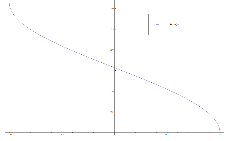
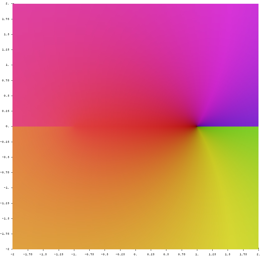
Put images into galleries. Thumbnails and frames break the theorem/proof box template. The code
<div align="center">
<gallery>
File:Arccos.png|Graph of $\mathrm{arccos}$ on $[-1,1]$.
File:Complex arccos.jpg|[[Domain coloring]] of [[analytic continuation]].
</gallery>
</div>
creates
Domain colorings
In Ubuntu... modify the cplot function in
/usr/lib/python2.7/dist-packages/mpmath/visualization.py
by commenting out the if statement at the end as follows:
    #if fig:
    #    if file:
    #        pylab.savefig(file, dpi=dpi)
    #    else:
    #        pylab.show()
This will allow us to call the savefig function ourselves as we do below. You may also alter the savefig command in visualization.py to have the correct parameters, but in most domain colorings we won't assume this.
With Python (best way)
We modify the code
#!/usr/bin/python
import numpy as np
import matplotlib.pyplot as plt
from mpmath import *

cplot(lambda sin(x): f(x),[-10,10],[-10,10],points=50000,verbose=True)
plt.savefig('complexsinedomaincoloring.png',bbox_inches='tight',pad_inches=0.0)
to generate domain colorings.
With Mathematica (old way)
We use the code
ComplexGraph[f_, {xmin_, xmax_}, {ymin_, ymax_},
  opts : OptionsPattern[]] :=
 RegionPlot[True, {x, xmin, xmax}, {y, ymin, ymax}, opts,
  PlotPoints -> 200, ColorFunctionScaling -> False,
  ColorFunction ->
   Function[{x, y},
    With[{ff = f[x + I y]},
     ColorConvert[
      Hue[(2. Pi)^-1 Mod[Arg[ff], 2 Pi], 1,
       1 - (1.2 + 10 Log[Abs[ff] + 1])^-1], "LAB"]]]]
to generate complex domain colorings. This coloring applied to the identity function $f(z)=z$ with the Mathematica code
 f[z_]:=z
ComplexGraph[f,{-10,10},{-10,10}]
Glyphs
When uploading a glyph (whether a plot in the plane or a domain coloring or a 3d graph), put[[Category:functionnameglyph]]in the description.
With Python (best way)
We use mpmath with the file visualization.py (in Debian, it is located at /usr/lib/python2.7/dist-packages/mpmath/visualization.py) altered in the following way: comment the two following lines
axes.set_xlabel('Re(z)')
axes.set_ylabel('Im(z)')
and add the following line
axes.set_axis_off()
Doing this will get rid of the left and right matter when using cplot. After this, use an image editing program (such as gimp) to cut out a square in the colored region. Upload this raw square with a filename like "complexsineglyph.png" (use prefix complex for domain colorings, without that prefix it should refer to a normal plot-type glyph) and upload that file.
$y=f(x)$-type graphs
#!/usr/bin/python
import numpy as np
import matplotlib.pyplot as plt
from mpmath import *
from pylab import rcParams
rcParams['figure.figsize'] = 2.4,2.4

x=np.arange(0,2*pi,0.00001)
f=np.vectorize(sin)
y=f(x)

fig, ax = plt.subplots()
plt.ylim([-1.1,1.1])
#ax.spines['left'].set_position('center')
ax.spines['right'].set_color('none')
ax.spines['bottom'].set_position('center')
ax.spines['top'].set_color('none')
ax.spines['left'].set_smart_bounds(True)
ax.spines['bottom'].set_smart_bounds(True)
ax.xaxis.set_ticks_position('none')
plt.tick_params(axis='x', which='both', bottom='off', top='off', labelbottom='off')
plt.tick_params(axis='y', which='both', left='off', right='off', labelleft='off')

plt.plot(x,y,linewidth=5,color='Black')

plt.savefig('sineglyph.png',bbox_inches='tight',pad_inches=0.0)
generates
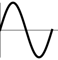
which we upload to the Wiki with name sineglyph.png. The file we get is  -- notice we have added the category
[[Category:sineglyph]]
This is so that we can use the randomimagebycategory extension.
Domain colorings
We use mpmath with the file visualization.py altered in the following way: comment the two following lines
axes.set_xlabel('Re(z)')
axes.set_ylabel('Im(z)')
and add the following line
axes.set_axis_off()
Doing this will get rid of the left and right matter when using cplot. After this, use an image editing program (such as gimp) to cut out a square in the colored region. Upload this raw square with a filename like "complexsineglyph.png" (use prefix complex for domain colorings, without that prefix it should refer to a normal plot-type glyph) and upload that file.
With Mathematica (old way)
We use the Mathematica code
Plot[AiryAi[x], {x, -12, 3}, PlotStyle -> {Thickness[0.04], Black}, AxesStyle -> Thickness[0.01], Ticks -> None]
to output the image
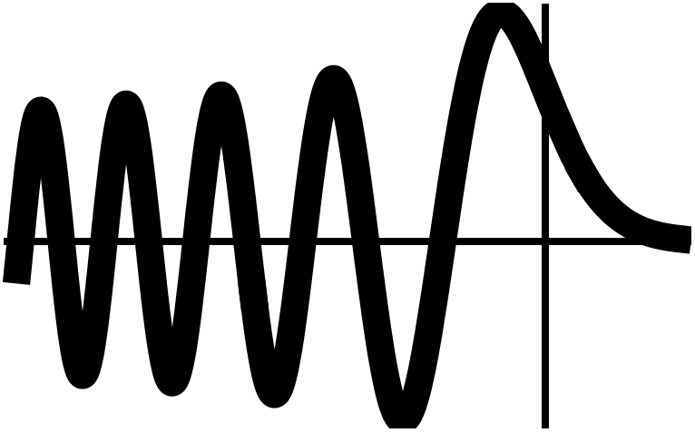
which we upload to the Wiki with name Airyaithumb.png use a thumbnail in an HTML table cell with the code
<td><center>[[File:Airyaithumb.png|45px|link=Airy Ai]]<br />
[[Airy Ai]]</center></td>
to display it.
Extensions
RandomImageByCategory
We use a modified version of RandomImageByCategory: inside RandomImageByCategory.php, replace the line
$thumbnail = "<a href=\"" . htmlspecialchars( $image_title->getFullURL() ) . "\">{$thumb_image->toHtml()}</a>";
with
$thumbnail = "{$thumb_image->toHtml()}";
This prevents RandomImageByCategory from forcing the generated image to link to the image itself and allows you make a randomly generated image link to another page using the following code:
[[Sine|<randomimagebycategory categories="Sineglyph" width="45" />]]
generates the randomly chosen image from the category Category:Sineglyph:
Categories
When uploading a traditional $x$-axis $y$-axis plot, use[[Category:Plot]]
When uploading a domain coloring, use
[[Category:DomainColoring]]
For any page for a specific special function, use
[[Category:SpecialFunction]]
When making a new theorem, use
[[Category:Theorem]]
If a theorem is proven, use
[[Category:Proven]]
If a theorem is not proven, use
[[Category:Unproven]]
If a theorem's proof requires more justification to be technically rigorous, then add the following category in addition to "Category:Theorem":
[[Category:Justify]]
Python LaTeX
Whenever we use Python to generate an image that contains LaTeX code, we have configured matplotlibrc with the following:
text.usetex : True
and
text.latex.preamble : \usepackage{amsmath}
